All code found in this blog post is also available on Google Colab where it can be executed directly in the browser.
When I first got interested in deep learning a couple of years ago, I started out using TensorFlow. In early 2018 I then decided to switch to PyTorch, a decision that I’ve been very happy with ever since. Today, the difference between the two frameworks is probably quite small in practice (and both are extensively used by researchers in the field), but I personally still find PyTorch more convenient to use.
In a short series of blog posts I thus intend to try and help anyone interested in the field to get started with PyTorch and deep learning, by providing (hopefully) clearly written code examples.
In this first post, we’ll start with perhaps the most simple example problem there is and try to fit a straight line to some noisy data points. We will however do so using mini-batch Stochastic Gradient Descent (SGD) and use the same basic code structure that can be used also for significantly more interesting problems, such as street-scene semantic segmentation or automotive 3D object detection.
Essentially, we need to specify just three things: a dataset class, a model class and a training loop.
Dataset
For our dataset class, we need to specify a constructor and two member functions.
In the constructor __init__, we create a synthetic dataset $D = \{(x_1, y_1), \dots, (x_N, y_N)\}$ by drawing $x_i$ uniformly from an interval and adding Gaussian noise to a given straight line:
\[
x_i \sim U[-3, 3], \quad i = 1, \dots, N,
\]
\[
y_i = \bar{k}x_i + \bar{m} + \epsilon_i, \quad \epsilon_i \sim \mathcal{N}(0, 0.5), \quad i = 1, \dots, N.
\]
We also assign the number of examples, $N$, to a member variable so that it can be returned by __len__.
Finally, in __getitem__ we return the corresponding example $(x_i, y_i)$ given an index $i \in \{1, \dots, N\}$.
import torch
import torch.utils.data

import numpy as np

import matplotlib.pyplot as plt

class LinearRegressionDataset(torch.utils.data.Dataset):
    def __init__(self, k, m, N):
        self.X = np.random.uniform(low=-3.0, high=3.0, size=(N, )) # (shape: (N, ))

        epsilon = np.random.normal(loc=0.0, scale=0.5, size=(N, )) # (shape: (N, ))

        self.Y = k*self.X + m + epsilon # (shape: (N, ))

        plt.figure(figsize=(8, 6))
        plt.plot(self.X, self.Y, "^k", label="Training data examples")
        plt.plot([-3, 3], [k*(-3)+m, k*3+m], "r", label="True straight line")
        plt.legend()
        plt.ylabel("y")
        plt.xlabel("x")
        plt.show()

        self.num_examples = N

        self.X = self.X.astype(np.float32)
        self.Y = self.Y.astype(np.float32)

    def __getitem__(self, index):
        x = self.X[index]

        y = self.Y[index]

        return (x, y)

    def __len__(self):
        return self.num_examples
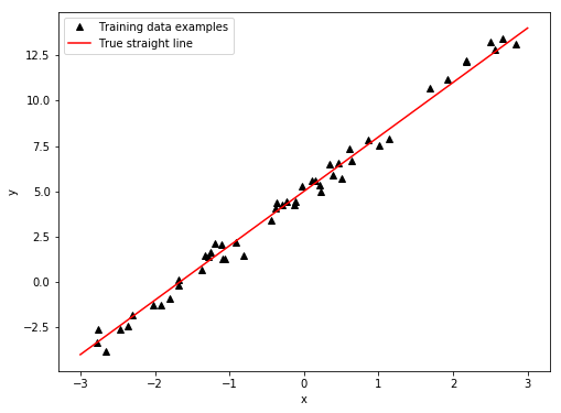
In __init__, we also plot our created dataset $D = \{(x_1, y_1), \dots, (x_N, y_N)\}$ together with the true straight line $y = \bar{k}x + \bar{m}$. For $\bar{k} = 3$, $\bar{m}= 5$, $N= 50$, we get the following plot:
Model
For our model class, we need to specify a constructor and one member function.
In the constructor __init__, we create our two model parameters $k, m$ and assign them to member variables. These are then used in forward to output a prediction $\hat{y} = kx + m$ for a given input $x$.
import torch.nn as nn

class LinearRegressionModel(nn.Module):
    def __init__(self):
        super(LinearRegressionModel, self).__init__()

        self.k = nn.Parameter(torch.zeros(1)) # (shape: (1))
        self.m = nn.Parameter(torch.zeros(1)) # (shape: (1))

    def forward(self, x):
        # (x has shape: (batch_size))

        y_hat = self.k*x + self.m # (shape: (batch_size))

        return y_hat
Training loop
To train our model on the dataset using SGD, we create instances of LinearRegressionDataset and LinearRegressionModel, we create the data loader train_loader (which will repeatedly call LinearRegressionDataset.__getitem__ to create mini-batches), and create the SGD optimizer object optimizer.
We then iterate through the entire dataset with mini-batches of size batch_size, and for each mini-batch we compute the L2 loss $L(k, m) = \frac{1}{N} \sum_{i=1}^{N} (y_i - \hat{y}_i)^2,$ we compute the gradients of this mini-batch loss with respect to our model parameters, and finally use these gradients in the SGD step to update the parameters.
One such iteration through the dataset is called an epoch, and we repeat this process num_epochs times.
from torch.autograd import Variable

num_epochs = 25
learning_rate = 0.01
batch_size = 8

k = 3
m = 5
N = 50

train_dataset = LinearRegressionDataset(k=k, m=m, N=N)

num_train_batches = int(len(train_dataset)/batch_size)
print ("num train batches per epoch: %d" % num_train_batches)

train_loader = torch.utils.data.DataLoader(dataset=train_dataset,
                                           batch_size=batch_size, shuffle=True,
                                           num_workers=1)

model = LinearRegressionModel()
model = model.cuda()
model.train() # (set in training mode, this affects BatchNorm and dropout)

optimizer = torch.optim.SGD(model.parameters(), lr=learning_rate)

epoch_losses_train = []
for epoch in range(num_epochs):
    print ("###########################")
    print ("epoch: %d/%d" % (epoch+1, num_epochs))

    batch_losses = []
    for step, (x, y) in enumerate(train_loader):
        x = Variable(x).cuda() # (shape: (batch_size))
        y = Variable(y).cuda() # (shape: (batch_size))

        y_hat = model(x) # (shape: (batch_size))

        loss = torch.mean(torch.pow(y - y_hat, 2))

        # optimization step:
        optimizer.zero_grad() # (reset gradients)
        loss.backward() # (compute gradients)
        optimizer.step() # (perform the SGD update of the model parameters)

        # store the loss value:
        loss_value = loss.data.cpu().numpy()
        batch_losses.append(loss_value)

    epoch_loss = np.mean(batch_losses)
    epoch_losses_train.append(epoch_loss)
    print ("train loss: %g" % epoch_loss)

plt.figure(figsize=(8, 6))
plt.plot(epoch_losses_train, "^k")
plt.plot(epoch_losses_train, "k")
plt.ylabel("Loss")
plt.xlabel("Epoch")
plt.title("Loss per epoch")
plt.show()

print ("k, true value: %g, estimated value: %g" % (k, model.k))
print ("m, true value: %g, estimated value: %g" % (m, model.m))

plt.figure(figsize=(8, 6))
plt.plot(train_dataset.X, train_dataset.Y, "^k", label="Training data examples")
plt.plot([-3, 3], [k*(-3)+m, k*3+m], "r", label="True straight line")
plt.plot([-3, 3], [model.k*(-3)+model.m, model.k*3+model.m], "b",
         label="Estimated straight line")
plt.legend()
plt.ylabel("y")
plt.xlabel("x")
plt.show()
In each epoch, we also store all mini-batch losses and then average them to get a loss value for the entire dataset. Once training is completed, we plot these epoch losses:
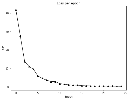
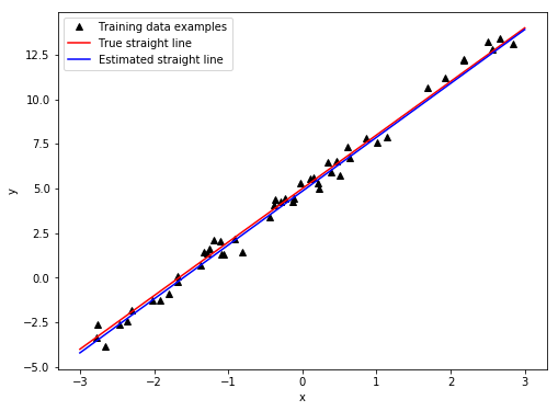
As we can see, the loss quickly decreases in the beginning and then starts to level out as our model parameters $k, m$ get close to the true values $\bar{k} = 3$, $\bar{m}= 5$. We also plot our estimated straight line $\hat{y} = kx + m$ and compare it to the true one:
Additional visualizations
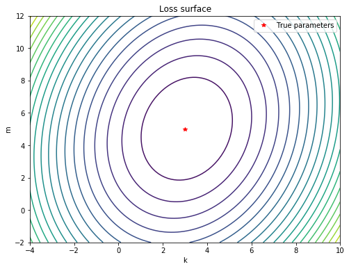
Since we in this simple example problem have just two model parameters, we can gain additional insight by computing our loss function $L(k, m) = \frac{1}{N} \sum_{i=1}^{N} (y_i - \hat{y}_i)^2$ (over the entire dataset) for different values of $k, m$ and plot the loss surface:
num_values=100
k_plot_values = np.linspace(start=(k-7.0), stop=(k+7.0), num=num_values)
m_plot_values = np.linspace(start=(m-7.0), stop=(m+7.0), num=num_values)
# (k_plot_values and m_plot_values both have shape: (num_values, ))
loss_values = np.zeros((num_values, num_values))
for k_i in range(num_values):
    for m_i in range(num_values):
        Y_hat = k_plot_values[k_i]*train_dataset.X + m_plot_values[m_i]
        # (Y_hat has shape: (N, ))

        loss = np.mean((train_dataset.Y - Y_hat)**2)
        loss_values[m_i, k_i] = loss

plt.figure(figsize=(8, 6))
K, M = np.meshgrid(k_plot_values, m_plot_values)
plt.contour(K, M, loss_values, levels=20)
plt.plot(k, m, "r*", label="True parameters")
plt.legend()
plt.ylabel("m")
plt.xlabel("k")
plt.title("Loss surface")
plt.show()
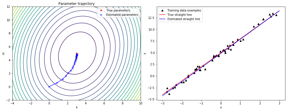
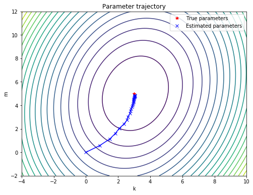
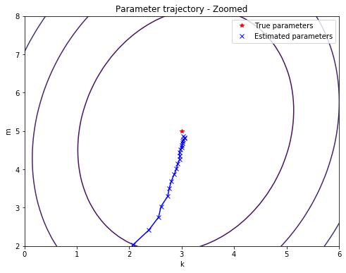
Finally, we can also store the current values of $k, m$ at different points during training and plot the parameter trajectory, starting at the initial point $(k_0 = 0, m_0 = 0)$ and ending at our final estimate $(k = 3.03, m = 4.86)$:
model = LinearRegressionModel()
model = model.cuda()
model.train() # (set in training mode, this affects BatchNorm and dropout)

optimizer = torch.optim.SGD(model.parameters(), lr=learning_rate)

epoch_losses_train = []
k_values = []
m_values = []
k_values.append(model.k.data.cpu().numpy())
m_values.append(model.m.data.cpu().numpy())
for epoch in range(num_epochs):
    print ("###########################")
    print ("epoch: %d/%d" % (epoch+1, num_epochs))

    batch_losses = []
    for step, (x, y) in enumerate(train_loader):
        x = Variable(x).cuda() # (shape: (batch_size))
        y = Variable(y).cuda() # (shape: (batch_size))

        y_hat = model(x) # (shape: (batch_size))

        loss = torch.mean(torch.pow(y - y_hat, 2))

        # optimization step:
        optimizer.zero_grad() # (reset gradients)
        loss.backward() # (compute gradients)
        optimizer.step() # (perform the SGD update of the model parameters)

        # store the loss value:
        loss_value = loss.data.cpu().numpy()
        batch_losses.append(loss_value)

    epoch_loss = np.mean(batch_losses)
    epoch_losses_train.append(epoch_loss)
    print ("train loss: %g" % epoch_loss)

    k_values.append(model.k.data.cpu().numpy())
    m_values.append(model.m.data.cpu().numpy())

plt.figure(figsize=(8, 6))
plt.plot(epoch_losses_train, "^k")
plt.plot(epoch_losses_train, "k")
plt.ylabel("Loss")
plt.xlabel("Epoch")
plt.title("Loss per epoch")
plt.show()

print ("k, true value: %g, estimated value: %g" % (k, model.k))
print ("m, true value: %g, estimated value: %g" % (m, model.m))

plt.figure(figsize=(8, 6))
plt.plot(train_dataset.X, train_dataset.Y, "^k", label="Training data examples")
plt.plot([-3, 3], [k*(-3)+m, k*3+m], "r", label="True straight line")
plt.plot([-3, 3], [model.k*(-3)+model.m, model.k*3+model.m], "b",
         label="Estimated straight line")
plt.legend()
plt.ylabel("y")
plt.xlabel("x")
plt.show()

num_values=100
k_plot_values = np.linspace(start=(k-7.0), stop=(k+7.0), num=num_values)
m_plot_values = np.linspace(start=(m-7.0), stop=(m+7.0), num=num_values)
# (k_plot_values and m_plot_values both have shape: (num_values, ))
loss_values = np.zeros((num_values, num_values))
for k_i in range(num_values):
    for m_i in range(num_values):
        Y_hat = k_plot_values[k_i]*train_dataset.X + m_plot_values[m_i]
        # (Y_hat has shape: (N, ))

        loss = np.mean((train_dataset.Y - Y_hat)**2)
        loss_values[m_i, k_i] = loss

plt.figure(figsize=(8, 6))
K, M = np.meshgrid(k_plot_values, m_plot_values)
plt.contour(K, M, loss_values, levels=20)
plt.plot(k, m, "r*", label="True parameters")
plt.plot(k_values, m_values, "xb", label="Estimated parameters")
plt.plot(k_values, m_values, "b")
plt.legend()
plt.ylabel("m")
plt.xlabel("k")
plt.title("Parameter trajectory")
plt.show()

plt.figure(figsize=(8, 6))
K, M = np.meshgrid(k_plot_values, m_plot_values)
plt.contour(K, M, loss_values, levels=20)
plt.plot(k, m, "r*", label="True parameters")
plt.plot(k_values, m_values, "xb", label="Estimated parameters")
plt.plot(k_values, m_values, "b")
plt.legend()
plt.ylabel("m")
plt.xlabel("k")
plt.xlim([k-3.0, k+3.0])
plt.ylim([m-3.0, m+3.0])
plt.title("Parameter trajectory - Zoomed")
plt.show()
Feel free to contact me or post a comment below if you have any questions or comments. In the next blog post, we’ll do nonlinear curve-fitting using feed-forward neural networks.